Don't Conform Your Data to the Model. Do the Opposite.

In this post, I'll be responding to an idea I saw on LinkedIn. See my guidelines on naming names.

The Problem

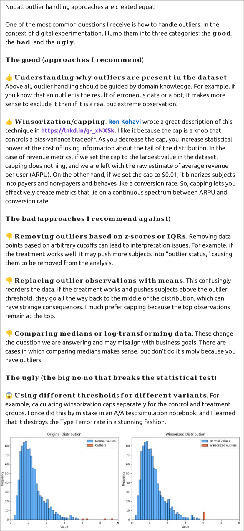
I recently saw a post on LinkedIn which serves as a nice example of how the null hypothesis mindset leads people to poor statistical decision making. The author works at an AB testing as a service company. Here is the post:

I agree with most of the points listed, but I want to focus on the suggestion to Winsorize the data and the plots at the bottom of the post.

The issue here is that the author wants to be able to compare the effect of a treatment on a continuous variable. The problem arises presumably because the author wants to conduct a two-sample t-test on the observations against a null hypothesis, but the skewed distribution of the observables will mean the assumption of normality on the sampling distribution of the means won't be valid at lower sample sizes, and hence will decrease the power of the test.

The Proposed Solution

Winsorizing is used to clip the highest values to reduce the skewness in the observed data; so instead of a long tail, the empirical distribution now has a small peak at whatever the threshold was.

If we suppose a frequentist null hypothesis test is what they want, there are problems with using a t-test here:

1. If we don't Winsorize the data, then the normality assumptions on the means do not hold until larger sample sizes (using CLT). So for sample sizes at which CLT does not apply (and what is that cutoff exactly?), the "frequentist guarantees" don't apply.
2. If we do Winsorize, then we've changed our data so the frequentist guarantees also don't apply. How could they? We're throwing out data so we won't have accurate estimates in the difference of our means.

The post frames this as a bias/variance trade-off. While this is better than insisting on unbiasedness above all else, it seems to ignore the typical reasons given for using the null hypothesis test in the first place: those guarantees.

Even if the method of analysis isn't a null hypothesis test, Winsorizing data still throws out information that might change our conclusion, had we not capped it. The value at which to cap it will necessarily be arbitrary. If we cap it ahead of time, then we may not know where a good cap is; if we cap it after the fact, how do we know our bias hasn't influenced the choice of cap?

In the Ron Kohavi post linked to in the screenshot, he discusses using the technique to reduce skewness and increase power. But increased power to compare what? If the continuous metric is what you care about, it's no longer clear what you're comparing with the new capped metric. He even gives an example of reducing required sample size by 50% through capping, and suggests capping at different levels to compare results. But how to decide which results to use? Maybe he explains it in his course that he links to, but it's hard to imagine a principled approach to deciding, and providing multiple options risks cherry-picking a convenient false positive.

The Alternative Solution

Instead of trying to make our data conform to the assumption of our model (the t-test relies on a model of the null hypothesis), we should do the opposite and find a model that describes the data well. Looking back at the post in the screenshot, we see an illustrative sample provided by the author. It looks like it would be well approximated by a log-distribution, and in my experience, this is quite common in revenue or customer lifetime value metrics. I agree with the author that we should not simply log the observations, but we could model the samples as log-normal distributions. Here are some benefits of doing so:

1. We don't throw out information. Assuming our measurements aren't flawed, we should try to retain all available information from these tests. Driving higher revenue value is valuable to the company. If we use the same Winsor cutoff on both samples, then whichever sample drove more users above the cutoff will be punished in the comparison.
2. The log-normal distribution naturally discounts the impact of outliers in the sample. It does this by estimating its parameters on the log scale. So we don't need to worry if one sample "got lucky" with a random draw far out in its tail; we won't be using its raw value in a mean calculation.
3. But this is different than just comparing the logged values. The mean of a log-normal distribution is a function of its log mean and standard deviation parameters: $\exp(\mu + \frac{\sigma^2}{2})$. So we can take into account how both the mean and spread of the distribution on the log scale impact the metric we car about in its original scale.
4. If the log-normal assumptions are a good match for the data, then it is a sample-efficient way to estimate the parameters.

Using Bayesian methods, we can estimate the parameters and create derived quantities using the equation above and have a posterior distribution over the difference, which we can use to estimate the probability of the treatment having a higher mean revenue or whatever we would like to know.

Of course, this may not work well in all situations; not all businesses have revenue distributions that are well modeled by log-normals. But perhaps other distributions will work well in those cases. When we conform our modeling assumptions to the nature of our data, we can make better comparisons about the things we care about in sample efficient ways. No need to cap.